It pretty much started here: McCulloch and Pitts wrote a paper [1] describing an idealized neuron as a threshold logic device and showed that an arrangement of such devices could express any propositional logic formula. Their neurons looked like this:

What this neuron does is fire if both of its excitatory inputs are active—unless the inhibitory input
(with the black dot) is active. McCulloch and Pitts would later go on to write a paper with Lettvin and Maturana [2] that showed how the neurons in a frog’s eye computed very specific environmental features.
These were exciting times: the Dartmouth AI conference had been held in 1956, with its promise of solving AI through symbolic methods. And didn’t the McCulloch-Pitts neuron have a symbolic interpretation as propositional logic? And weren’t those features detected by a frog’s eye themselves some kind of logical propositions? Was there some kind of grand synthesis immanent?
Not right away. One of the problems with these threshold logic circuits was that they had to be hand-designed, yet neurons in the brain seemed to learn on their own. Into this world came Frank Rosenblatt [3,4], who proposed the Perceptron:
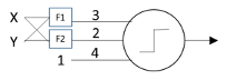
Like the McCulloch-Pitts neuron, the Perceptron is a threshold logic device, but there are some differences. First, inputs and outputs are now not merely denoted as “active” or “inactive” but are explicitly represented by 1 and 0, respectively. Second, now math happens: each of the Perceptron’s inputs gets multiplied by a weight (the values 3 and 2 in the figure above). Third, the threshold value (4 in the figure above) has been moved onto a bias input, which has a constant input of 1: when the weighted sum of its two inputs is larger than its bias weight, this neuron will fire. Fourth—and most importantly—all of these weights are learned autonomously.
This was a big deal. Before the Perceptron, it wasn’t clear that any learning procedure would actually converge to a correct answer. As it turns out, if two classes are separable in feature space (in this case, the two-dimensional space defined by the two outputs of the feature detectors F1 and F2 shown above), the Perceptron can learn to distinguish the two classes. Whether this kind of simple circuit actually worked depended on the feature detectors, which—unlike the Perceptron weights—were handcrafted, not learned. Although only two feature detectors are shown here, there can in fact be arbitrarily many of them, and they can be made arbitrarily complex.
Rosenblatt wasn’t the only one at that time with a learning procedure in the guise of a neural model: Bernard Widrow and Marcian Hoff introduced the Adeline [8], shown here.
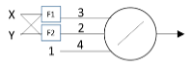
The Adaline differed from the Perceptron in several ways. Most importantly, its output was not thresholded but was simply the linear weighted sum of its inputs. Also, in order to make this work, the presence of a feature on its inputs was no longer represented by 0 and 1, but by -1 and 1, respectively. This meant that its output was not simply a binary 0 or 1, but ranged over all real numbers. When used as a classifier, the convention was that a negative or zero output signified “not in class” and a positive signified “in class”. Another important difference was its learning rule, which was adjusted the input weights along an error gradient based on the least-squared error of its output.
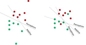
The Adaline allowed you to do classification when the classes were not linearly separable, a situation where a Perceptron would fail. This is shown below. On the right are a pair of classes that are not linearly separable. The Adaline has done a reasonable job of finding a line to discriminate between them in most of the cases, but the Perceptron cannot converge to any kind of stable solution. But even so, the Adaline was not guaranteed to find a linearly separable solution even when one existed. This is shown on the left, where the Perceptron has correctly separated the classes, but the Adaline, under the influence of squared-error from outliers, has been pulled away from such a solution.
Apparently, Rosenblatt overhyped his work, or at the very least annoyed Marvin Minsky and Seymour Papert, who wrote a book that emphasized negative results about perceptrons [5]. They were not wrong: the results they found about the limitations of perceptrons still apply even to the more sophisticated deep-learning networks of today. However, between the lines of “Perceptrons”, you can detect a certain snippiness and glee as they downplay Rosenblatt’s work. This book effectively killed off interest in neural networks at that time, and Rosenblatt, who died shortly thereafter in a boating accident, was unable to defend his ideas. (I once heard that Minsky much later regretted having been so harsh on Rosenblatt’s work. So it goes.)
Around this time a new graduate student, Geoffrey Hinton, decided that he would study the now discredited field of neural networks. We’ll hear more about him in a bit.
A few years later, a much less distinguished scholar also decided to also make the career-killing move of studying neural networks. When I arrived at the University of Massachusetts at Amherst in 1983, I took a course on neural networks with Andrew Barto. The papers were a curious hodge-podge from researchers who, like Geoff Hinton, were trying to keep the faith, but there was no unifying theory behind them. We were definitely in a Kuhnian pre-paradigmatic period. This would change in 1986 with the publication of “Parallel Distributed Processing” [6], which included a description of the backpropagation algorithm [7]. (Note that Geoff Hinton was a co-author on this paper: his interest in neural networks was finally vindicated. It would not be the last time that happened.)

The figure above shows a back-propagation network. It looks a lot like the Perceptron except that the thresholding function has been replaced by a differentiable approximation to the threshold function (which we all adorkably called “the squashing function”), and the F1 and F2 handcrafted feature detectors have been replaced by still more back-propagation units that can actually learn the features from training examples. In principle, you could have as many of these additional units as you wanted, arranged in as many layers as you wanted, with as many units in each layer as you wanted. And in theory, you were guaranteed to be able to learn anything. In fact, it was shown that it would take only three layers—including the input layer—to be able to approximate any function using a neural net [10].
What made the back-propagation unit different was that—unlike the Perceptron, with its nondifferentiable threshold function—you could calculate the derivative ∂ Err/∂wi for each weight wi of the unit, which told you by how much you should change the weight to decrease the output least-squared error (the very same error used in an Adaline). What’s more, you could also calculate ∂Err/∂xi, which indicated how much a given input contributed to the output error. This value would be passed back to the unit supplying the input, which would use it to adjust its weights and pass error gradients back to the units supplying its inputs, and so on, allowing weights to be adjusted recursively throughout the network.
In retrospect, this algorithm seems obvious, and perhaps it was. Andy Barto once remarked that he and many of his colleagues had thought of this algorithm themselves but never bothered to investigate it because it was clear that it would never work. Others, such as Paul Werbos [11], had in fact actually published the algorithm but had been ignored by the neural network community. (In fairness, once Werbos’ contribution was pointed out, the neural network community started citing his work. It probably didn’t hurt that he was also the guy handing out funding at the NSF.)
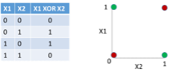
To understand the excitement around the backpropagation algorithm, we need to take a look at the
XOR problem, shown above as a logical truth table and its two-dimensional feature space. A single-layer Perceptron or Adaline (that is, single units with no hand-crafted feature layer between them and their raw inputs) are both called linear classifiers because their decision is made by computing a linear function, the weighted sum of their inputs. Recall that they draw a line in the feature space that either cleanly separates the red and green points in the space or at least separates them in a way that puts most of them are on the correct side of the line. As you can see above, there is no way to draw a line in the XOR feature space below that cleanly separates the red from the green points (Perceptron) or puts the majority of the red and green points on the correct side of the line (Adaline). Both the single-layer Perceptron and Adaline would utterly fail at implementing the very simple logical formula shown in the truth table.
But the multilayer backpropagation network could do XOR easily! It is hard to overestimate the shock and awe that went through the neural network community around this simple example. It felt like the discovery of fire. Soon many papers appeared that applied backpropagation networks to real-world problems. For example, Dean Pomerleau used them to create a system that learned to drive a car [12]. (I can personally confirm that this more or less worked. While working as an RA in the computer vision group, I had the opportunity to sit in a robotic Humvee as it used Pomerleau’s code to drive around the University of Massachusetts’ stadium.) This was a good time to be doing research in neural networks: an ambitious, strategic, energetic graduate student could get a dissertation completed quickly while making some kind of contribution to the field.
This scholar was not that kind of grad student. I had the opportunity to be working alongside some people who were or would become luminaries in this field, such as Andy Barto and Rich Sutton, who thought deeply about reinforcement learning [122] and would frame the discussion going forward, and Mike Jordan, an enfant terrible who had a wide range of interests, but who would soon steer the conversion away from neural networks and towards Bayesian networks and other graphical models [68]. However, I wasn’t particularly interested in researching learning per se; instead, I was much enamored by distributed knowledge representations.
If you read papers from that time [13–16], there was a fascination with how a neural net activation pattern might somehow encode many facts about a thing “subsymbolically”. That is, in a traditional symbolic AI system, a token by itself is just a symbol with no implicit meaning: it acquires its meaning through chains of connections to other tokens. For example, the symbol “apple” might be linked to the symbol “red”. In contrast, in a neural network, the pattern of activation for “apple” might contain a subpattern that somehow represented “red”. Everyone seemed to have their own theory around how this might work, so we clearly were living in a pre-paradigmatic era for subsymbolic representation. Nevertheless, in the second volume of the PDP book [17], I found an approach to place recognition I rather liked (the-image-is-the-place) [20], so I turned my attention to robot navigation [19]. I was out of the neural net biz.
Fast-forward a couple of decades: I was (and still am) working at Lexalytics, a text-analytics company that has a comprehensive NLP stack developed over many years. Initially, we had been using classic symbolic NLP algorithms, but in recent years we had started to incorporate machine learning (ML) models into more and more parts of our code, including our own implementations of conditional random fields [11] and a home-grown maximum entropy classifier. Going forward, it was clear that we would need to be supporting even more models across more languages, yet our code and training data were scattered across many cloud computing instances. This annoyed me, so I created a RESTful service that would allow us to aggregate the model creation code and data all in one place.
Around this time (early 2016), our management team realized that to maintain relevance as a company, we would need to be able to incorporate even more ML into our product. Paul Barba and Al Hough vastly expanded the technical vision around the model creation system, and Al Hough took on the task of turning the rudimentary RESTful service into a robust, extensible, production-grade system for generating state-of-the-art ML models. The engineering team also started a weekly reading group, studying recent machine learning papers so we could come up to speed and remain current on the start of the art. And when I started reading these papers, the first question that came to my mind was:
Dude, where’s my neural net?!?
Gone were the lovingly crafted figures of the neural network architectures and the philosophical asides about subsymbolic representations: in their place were just complex cost functions to be minimized. It felt a lot like the shift in the early days of quantum theory from discussions of the meaning of quantum theory to the Copenhagen interpretation, with its injunction to just “shut up and calculate”. In this case, it was more like “shut up and optimize”.
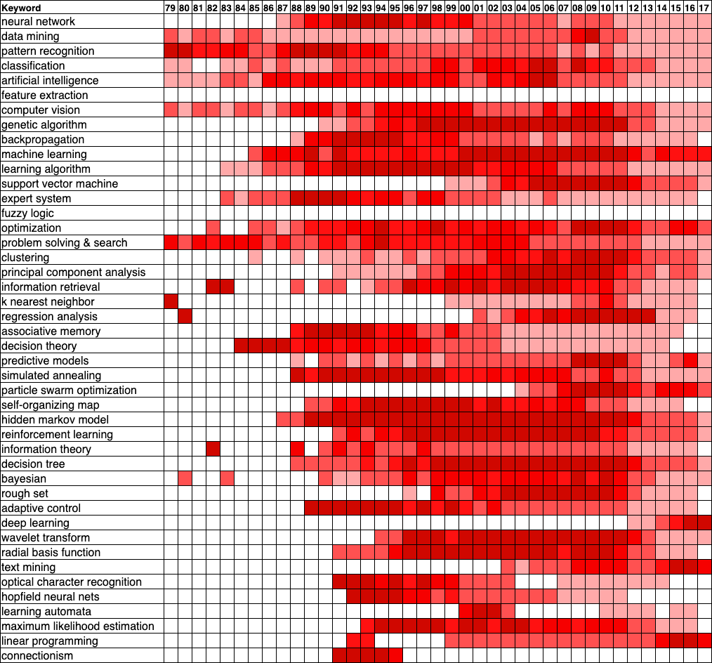
This subjective impression is objectively backed up by the heat map below, constructed from a dump of the Microsoft Academic Graph (MAG) circa 2017 [21]. To create this heat map, I selected a subset of documents from the field of study “Machine Learning” and then looked at the backward and forward references starting from a set of well-known machine learning papers. From these, I selected the top 300 keywords by their maximum document frequency over their lifetime (their “mindshare”, if you will). From these, I dropped keywords that were too general or irrelevant and merged keywords that more or less meant the same thing. The mindshare of each keyword is normalized over its lifetime, so 0% mindshare is displayed as white and 100% of the keyword’s maximum mindshare is displayed as very dark red. In the heat map, the keywords are arranged from top to bottom in decreasing order of their maximum mindshare over their lifetime.
What we can see is that terms like “neural networks” and “backpropagation” are popular in the ’80s and ’90s, but fade out thereafter. Even more embarrassingly, the keyword “connectionism”, which came out of the PDP group [6,17] and was intended to mark the territory for the new paradigm of subsymbolic AI, died ignominiously after a few years. And indeed we can see other machine learning topics arising to take their place, like “optimization” in the mid-’00s, with “deep learning” springing out of nowhere in 2012.
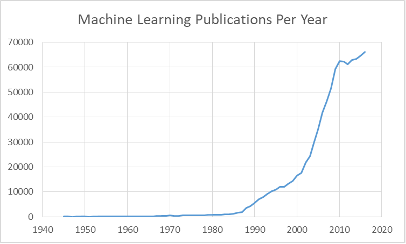
So, whatever did happen to neural networks? The graph below shows the trend of publications in machine learning. What jumps out at us is an inflection point in the mid-to-late ’80s and another one in the early ’00s. (Ignore the plateau around 2010: this is probably an artifact of the incompleteness of the MAG dump.) The first inflection point is almost certainly due to the renewed interest in neural networks, thanks to the introduction of the backpropagation algorithm. You can see that after 1987, keywords for other type types of learning algorithms, such as hidden Markov models [22], decision trees [23], Bayesian networks [25], and support vector machines (SVM’s) [24], begin to be mentioned or mentioned more. This certainly contributed to the fading of mentions of “neural network” since the appearance of all these new topics could only serve to dilute its document frequency.
Yet this cannot be the complete answer to the apparent waning of neural networks, since these other new techniques certainly did not seem to cannibalize each other’s mindshare. Another perspective is offered by LeCun, Bengio, and Hinton [26]:
“In the late 1990s, neural nets and backpropagation were largely forsaken by the machine learning community and ignored by the computer-vision and speech-recognition communities. It was widely thought that learning useful, multistage, feature extractors with little prior knowledge was infeasible. In particular, it was commonly thought that simple gradient descent would get trapped in poor local minima — weight configurations for which no small change would reduce the average error.”
And Simard, Steinkraus and Platt [27] say:
“After being extremely popular in the early 1990s, neural networks have fallen out of favor in research in the last 5 years. In 2000, it was even pointed out by the organizers of the Neural Information Processing System (NIPS) conference that the term “neural networks” in the submission title was negatively correlated with acceptance.”
If we take them at their word, the behavior of the machine learning was driven by a communal belief that learning in multilayer perceptrons was infeasible—a recycled version of the pre-1985 belief that multilayer perceptrons would never work. This time around, though, there was a little more empirical justification for this belief. Simard et al [27] found that “the MNIST database [for handwritten digits] is too small for most algorithms to infer generalization properly”. Although the neural networks of the ‘80s worked well for toy problems (a small-data, small-feature regime), they did not work well with real-world problems. But it wasn’t a matter of poor data: rather, there was not enough data available to be able to infer a large enough set of useful features. The networks were hampered because they were working in a small-data regime.
In the case of Simard et al [27], they got around this problem by augmenting the MNIST data set by subjecting the images to many elastic transformations, turning it into a large-data regime that allowed them to get good results. Nevertheless, this trick couldn’t be applied to all problem domains. And this gives us a clue to the second inflection point in the graph above.
As we spend our days compulsively checking our smartphones, it may be hard to remember that we were not always so connected. The dot-com boom followed by the dot-com bust in 2000 left the world massively wired with fiber optics and allowed Google to acquire scads of defunct data centers at firesale prices [29], giving them the resources to truly index everything. And as other online companies began to recover and other companies began to move their services online, they developed the need to exploit their customer data. We had entered the time of big data and the need for algorithms that could work with it. I propose that this is what drove the second inflection point.
| Deep Learning Timeline: Classifier Cage Match <2001 – 2005 | |||
| Year | Algorithm | Application | Library or Database |
|---|---|---|---|
| Before 2001 | Long Short-Term Memory
(LSTM) [108]; Convolutional Neural Nets [107] |
MNIST Handwritten Digit DB [28] | |
| 2001 | Random Forests [30]; Statistical Learning [31]; Evolutionary Algorithms [38]; Conditional Random Fields [32]; Support Vector Machines [33]; Matrix Factorization [35]; Bayesian Networks [36]; Principle Components Analysis [37]; AdaBoost [40]; Markov Random Field [39]; Convolutional Neural Nets [34]; |
Collaborative Filtering [42]; Face Detection [43] |
|
| 2002 | Latent Dirichlet Allocation [48]; Hidden Markov Models [46]; Boosting [44]; Discriminative/Generative Classifiers [114]; Ensemble Methods [47] |
Data Mining [45] | MALLET Software Library [41] |
| 2003 | Feature Selection [49]; Markov Chain Monte Carlo [52]; Maximum Likelihood Estimation [53]; Word Vectors [51]; |
Machine Translation [50]; Language Model [51]; Named Entity Recognition [54]; Part-of-Speech Tagging [55]; Handwriting Recognition [27] |
|
| 2004 | K-Nearest Neighbors [56] | Image Features [56]; Sentiment Analysis [57]; Text Summarization [58]; Topic Models [59] |
NORB Image DB [109] |
| 2005 | Clustering [60]; | Recommendation Systems [61]; Human Detection [62] |
|
| Deep Learning Timeline: Deepness Arising 2006-2008 | |||
| Year | Algorithm | Application | Library or Database |
|---|---|---|---|
| 2006 | Deep Belief Networks [64]; | ||
| 2007 | Deep Networks [65]; Transfer Learning [66]; |
||
| 2008 | K-Nearest Neighbor [72]; Fuzzy Logic [73]; LargeScale Learning [74]; Deep Networks [76] |
Natural Language Processing [76]; Data Visualization [77] | LIBLINEAR Software Library[67] |
| Deep Learning Timeline: Deep Domination 2009 onward | |||
| Year | Algorithm | Application | Library or Database |
|---|---|---|---|
| 2009 | Dimensionality Reduction [69]; Deep Learning [78] |
||
| 2010 | Transfer Learning [70]; Rectified Linear Units [71]; Denoising Autoencoders [75]; Unsupervised Pretraining [78]; Stochastic Gradient Descent [82]; Deep Learning Convergence [83] |
ImageNet Image DB [86] | |
| 2011 | Natural Language Processing [105] | LIBSVM Software Library[79]; Scikit-learn Software Library [80] |
|
| 2012 | Deep Convolutional Neural Networks [84] | Image Recognition [84] | |
| 2013 | Word Vectors [85,87]; | ||
| 2014 | Dropout [89]; Word Vectors[90]; Long Short-Term Memory (LSTM) [91] |
Machine Translation [91] | Caffe Software Library [88] |
| 2015 | Deep Convolutional Neural Networks [92,93]; Batch Normalization [94]; Adam Optimizer [95]; |
||
| 2016 | Residual Learning [97]; LSTM [98] |
Machine Translation [98] | TensorFlow Software Library [96] |
| 2017 | Transformer [99]; Capsules [101] |
||
| 2018 | Regularization [100]; ELMo [102]; BERT [103] |
||
| 2019 | GPT-2 [104] | ||
| 2020 | GPT-3 [105] | ||
The timeline above zooms in on the work that was being done around the time of the second inflection point and thereafter The timetable was generated by looking at the 1000 most-referenced articles since 2000 in the MAG database, then sorting them first by year, then by citation count. For each year I looked at the top most-cited articles and entered the article’s topics if they had not already appeared in the timeline for a previous year. (This is why the timeline seems so front-loaded for the earlier years.) Since the MAG database petered out around 2017, I filled out the rest of the timeline with topics I knew were important. Topics particular to deep learning are boldfaced.
The boldface more or less divides this timeline into three eras: 2001-2005, Classifier Cage Match; 2006-2008, Deepness Arising; 2009 onward, Deep Domination. The Classifier Cage Match era was a time of algorithms scrabbling for dominance in a small-data, small-feature regime. This characterization can be inferred from the timeline by noticing the image databases, which were all small by modern sizes. And the large data that drove the Netflix Prize Challenge would not be released until 2006 [110], the beginning of the Deepness Arising era.
A paper that exemplifies the Classifier Cage Match era is LeCun et al [109], which pits support vector machines (SVMs), k-nearest neighbor (KNN) classifiers, and convolution neural networks (CNNs) against each other to recognize images from the NORB database. The CNN was a 6-layer neural net with 132 convolution kernels and (don’t laugh!) 90,575 trainable parameters, placing it in the small-feature regime. KNN was a well-established classification algorithm, and SVM was a recent upstart that had become the go-to algorithm of choice for classification. Let’s take a closer look at each of these to understand why they prospered in a small-data regime.

The image above shows the now-familiar set of red and green points in a two-dimensional feature space. How do you suppose the point at the “?” in this feature space should be classified? You probably have a sense that it should be classified as “green”—even though it is closest to a red point—because most of its neighbors are green. This is exactly what a k-nearest neighbor classifier does. It doesn’t need much data: just enough to sketch the shapes for the general outlines of the classes, in this case, “red” and “green”. So, KNN algorithms were well-suited for a small-data regime.
As were SVM’s. Recall the XOR problem mentioned previously? There was no way to draw a line that would separate the red from the green points. But what if we added a third feature X1 AND X2, the logical combination of the features X1 and X2? The feature space now becomes three-dimensional, as shown below. As you can see, the extra dimension (i.e., feature) raises one of the red points above the other three. Now we can easily separate the red from the green with a slanted plane (the light blue triangle, extended infinitely on all of its sides): the red points lie above this plane and the green points below.
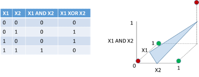
The XOR problem is a particular example of the single-layer Perceptron butting heads with its “VC-dimension”. The best way to think of the VC-dimension is to ask yourself, “What is the minimum number of points needed to foil this classifier, at least some of the time?” The VC-dimension will be one less than this number. Since it took four points in the two-variable XOR arrangement to fool the original two-input Perceptron, that Perceptron had a VC-dimension of only 3. However, adding another dimension by way of the feature X1 AND X2, we created a Perceptron with a VC-dimension of 4, so it could no longer be fooled by the two-variable XOR problem.
This is one of the “tricks” behind the SVM, invented by Vapnik (the “V” in “VC-dimension”) [24]. The SVM makes use of inner-product kernels that implicitly increase the number of features (i.e., dimensions)…even to an infinite number of them! This yields an infinite VC-dimension, which means an SVM classifier can’t be foiled by any number of data points. So how do you multiply an infinite number of inputs by an infinite number of weights? You make use of the so-called “kernel trick”: the implementation of the SVM merely requires the result of this weighted sum, not the infinite number of individual products themselves. As it turns out, these inner products of kernels can be implemented as closed-form mathematical expressions. A third trick behind the SVM is how it optimally positions its separating hyperplane, make it equally distant from two classes. This gives it a better shot at generalization. Even when the data are not separable, an SVM can converge to a useful answer: this is its fourth trick. In short, it combines the best of both the Perceptron and the Adaline. Since the SVM only cared about the few points near the boundaries of the classes, it worked well with small amounts of data.
What’s missing from both KNN and SVM is any mechanism for automatic feature selection. As you can see from the timeline, “feature selection” was still an issue in the Classifier Cage Match era. And it wouldn’t do to simply generate an arbitrarily large number of different arithmetic and logical combinations of the raw input features to be used in these algorithms. For KNN, using a large number of superfluous dimensions (features) might have scattered the data points so that former nearest neighbors became widely dispersed. For SVM, using a kernel with a large VC-dimension might have guaranteed the separation of the classes, but at the expense of generalization. Features still needed to be hand-engineered, which meant that these algorithms still operated in the small-feature regime. And although the CNN used by LeCun et al [109] did learn its own features (parameters), it had just a small number of them by today’s standards. But all of that was about to change.
In 2006, Hinton et al [64] (yup…Hinton again) published an algorithm for what they called a “deep belief network”, where they used unsupervised learning to pre-train a multilayer network one layer at a time. It worked like this: big images were fed into a much smaller layer of learning units that were trained to reproduce the images on their outputs. This layer performed data compression on the images—essentially extracting its salient features. And because the goal of the training was simply to be able to reproduce the layer’s input—which was known—there was no need to use a data set that had to be laboriously curated and labeled by humans. It was possible to make use of as many raw images as it could get its hands on.
After the first layer was trained, the images were fed through the first layer into a second layer, which was trained to reproduce the input image (while the features of the first layer were held unchanged). The second layer formed higher-level features composed of the lower-level features from the first layer. Then the second layer was attached to a third layer that was trained to reproduce the input (while the first and second layers were held unchanged), forming even more complex features. In the end, there were three hidden layers and 1.7 million weights. It was the beginning of the large-feature regime in machine learning.
The Deepness Arising era had begun, though this is only clear in retrospect. Many of the papers published with “deep” in their title were authored by a just small group of people, typically Hinton, LeCun, Bengio, and their students. And there was pushback, as advocates of other algorithms such as K nearest neighbors [72] and fuzzy sets [73] published papers arguing about why you should not count them out just yet.
The Deepness Arising interregnum lasted only until it was shown that this layer-by-layer pre-training approach could produce a killer app that could be monetized, namely a speech recognition to be installed on cellphones [26,112,113]. This began the era of Deep Domination. Not only were we now living in the large-data, large-feature regime, but we were also feeling very…comfortable…in it. And in 2012, Alex Krizhevsky, Ilya Sutskever and Geoffrey E. Hinton (again!) found that deep learning could do away with pre-training entirely and directly use good, old-fashioned convolutional neural networks (CNNs), with some enhancements [84] :
“When deep convolutional networks were applied to a data set of about a million [ImageNet] images from the web that contained 1,000 different classes, they achieved spectacular results, almost halving the error rates of the best competing approaches. This success came from the efficient use of GPUs, [rectified linear units], a new regularization technique called dropout, and techniques to generate more training examples by deforming the existing ones. This success has brought about a revolution in computer vision; [CNNs] are now the dominant approach for almost all recognition and detection tasks and approach human performance on some tasks.” [26]
It is hard to overstate how jaw-dropping this result was. As someone who has worked in computer vision in academia and industry over the years, I can attest that we had always struggled to create any kind of image understanding algorithms that would perform well. And here a machine learning approach was eating our lunch.
These early successes of deep learning mostly concentrated in the domain of images. This is not surprising, since visual perception is one of the main modalities of human experience and communication. But the other big modality is human language, especially as captured in text. Indeed, some of the killer apps in the early Internet years were search engines, and it is fair to say that the Internet would not be remotely useful without them.
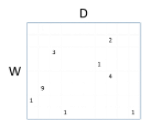
The word-document matrix above schematically represents what is (conceptually) done under the hood of a search engine. It keeps track of how many times a word (indexed by a row in the matrix) appears in a particular document (indexed by a column in the matrix). As you can see, the matrix is sparse: most words don’t appear in most documents, and most documents don’t contain most words. And realize that this matrix is just a tiny conceptualization: the real matrix would have millions of columns (documents) and tens of thousands of rows (words).
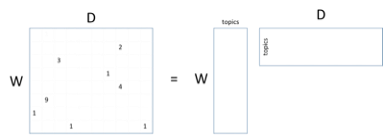
Using latent Dirichlet allocation (LDA) [114,115], it is possible to factor a word-document matrix into the matrix product of two other matrices: the word-topic matrix and the topic-document matrix, as shown above. In the topic-document matrix, each document is represented by a very concise topic vector with the property that if two documents are talking about the same topic, their topic vectors will be similar. This is just the sort of representation that is useful for a search engine. However, a similar thing holds true for the word-topic matrix: if two words have similar meanings, their topic vectors will be similar. This is the sort of representation that is useful for natural language processing.
A drawback to this approach for encoding word meanings from documents is that a document can be about many topics, so the meaning of their word-topic vectors can be a little bit fuzzy. We can address this by restricting our attention to just a small context of words surrounding each word in each document. For example, in the sentence “I gave my dog a bone”, the four-word context for the word “dog” would be “gave my a bone”. From words with their contexts, we can create a word-context matrix and its factorization [116].
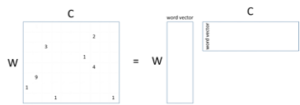
This looks just like the word-document factorization except that the columns now represent contexts (C) rather than documents. And this is what was done by Mikolov et al [85] with their word2vec algorithm, which produced (as you would guess) the word/word-vector matrix. Not only did words with similar meanings have word vectors that were close to each other, but the meanings of the words also seemed to be accessible through simple vector arithmetic. The famous example from this paper was [king] – [man] + [woman] = [queen]. That is, subtracting the word vector for “man” from that of “king” seemed to produce the meaning “royalty”, so that when you added it to the word vector for “woman” you got “queen”.
This was yet another jaw-dropping moment in the Deep Domination era and one that seemed to finally fulfill the dream of subsymbolic representations from the 1980s. Yet there was still a problem with these kinds of word vectors: a word could have only a single word vector, yet sometimes a given word could mean different things, e.g., “bank” as a financial institution versus “bank” as the side of a river. Somehow the representation of a word in a document also had to drag along some aspect of its context so that it represented the correct sense in which it was being used.
The path to a contextual interpretation of words lay in language models. The idea of a language model is that given a fragment of text or an utterance, the model could predict what word would come next. In a sense, the word vector/context matrix shown above is a kind of language model: given the context of a few words, you can predict the word vector for the word in that context. But conventionally a language model is trained to produce the next word in a document given the sequence of words seen so far.
The neural network architecture that comes naturally to mind for learning a sequential language model is a recurrent network, where the internal state of the network—a compact representation of the sequence of words seen so far— is fed back into the network as an input to predict the next word. Unfortunately, recurrent neural networks proved very hard to train [9]: backpropagation error gradients would either disappear (making learning slow or impossible) or explode (making learning unstable). Hochreiter and Schmidhuber [108] found a way to address these gradients with their long short-term memory (LSTM) architecture. The innovation of the LSTM is that it interposed a trainable, multiplicative layer between the internal state from the previous time step and the current time step, enforcing a constant error flow through the internal states. This allowed the LSTM to bridge time intervals of over 1000 time steps.
But even with tools like the LSTM, learning language models with recurrent networks was still considered difficult [117]. Nevertheless, Sutskever et al [91], using a pair of 5-layer LSTMs, were able to construct an English-to-French translator, where one LSTM served as an encoder and the other as a decoder. The encoder produced a compact vector representation of the entire input sentence, which the decoder used to generate the sequence of output words. The final result was chosen using an ensemble of these encoder-decoder pairs.
This result was impressive enough to make it one of the top 1000 cited papers in the timeline, but the surprising innovation in encoder-decoder architectures came about three years later. The Transformer [99] eschewed recurrent networks and instead held its entire input in a buffer. Its inputs were preprocessed in a way that encoded their positions within the sequence. But the real innovation was its method of learning several windows of attention into different parts of the input sequence, which allowed it to pick the ideal context for disambiguating the meaning of a word in its input sequence. And since the Transformer was a 6-layer network, its attention units at each level allowed it to operate over more and more complex semantic features of the input sequence. At the time, its performance in translating from English-to-German and English-to-French surpassed all previously published models.
Around the same time, ULMFiT [119] showed how to effectively do transfer learning to incorporate a hard-won language model into any NLP learning task, and ELMo [102] showed how it was possible to do the same with a deeply contextualized language model built around LSTMs. ELMo would also be the first of the Muppet-themed language models that would come to include ERNIE [120], Grover [121]….and BERT.
BERT. The base model of BERT [103] had 12 (!) layers of bidirectional Transformers. If you gave BERT a chunk of input text, it produced word vectors that encoded each word’s context, so that now it was finally possible to disambiguate “bank” (the financial institution) from “bank” (the edge of a river). As with ULMFiT and ELMo, these contextual word vectors could be incorporated into any NLP application. And what’s more, Google made BERT publicly available, so that everyone could have access to contextual word vectors.
It’s time to use the word “jaw-dropping” again. To get a sense of just how well BERT performed, shortly after BERT was released, Lexalytics attended a data science colloquium where many of the presenters talked about how they were switching over to BERT in their research. Some of them were dropping work they had been laboring on for years. BERT is just too good not to use. In fact, Lexalytics has incorporated BERT into our text analytics engine.
A couple of main contenders to BERT’s pre-eminence as a contextual language model are GPT-2 [104] and GPT-3 [105]. A recent paper [118] that made use of GPT-2 tracked the neural activity from electrodes implanted in people’s brains as they listened to spoken text. The researchers tracked neural patterns that anticipated the next word to be read and compared it to the word vector predicted by GPT-2. They discovered that there was a linear transformation between the neural patterns and the GPT-2 word vectors. It seems that our brains are using something much like contextual word vectors.
There is something satisfying about this, in a poetic justice sense. Starting from the overly simplified canonical model of neurons, the McCullough-Pitts threshold logic unit, we passed through a period of exuberant hope that computer science could provide deep insights into neural computation, a hope that apparently became so embarrassing in its naiveté that the whole research direction was shunned for a while. Yet now we find that contextual representations like those created by modern-day neural networks seem to be showing up in the brain.
A circle has been closed.
References
- Warren S. McCulloch and Walter H. Pitts (1943) “A Logical Calculus of the Ideas Immanent in Nervous Activity”
- Y. Lettvin, H. R. Maturana, W. S. McCulloch and W. H. Pitts (1959) “What the Frog’s Eye Tells the Frog’s Brain”
- Frank Rosenblatt (1959) “Two Theorems of Statistical Separability in the Perceptron”
- Frank Rosenblatt (1962) “Principles of Neurodynamics”
- Marvin Minsky and Seymour Papert (1969) “Perceptrons: An Introduction to Computation Geometry”
- James L. McClelland, David E. Rumelhart and the PDP Research Group (1986) “Parallel Distributed Processing: Explorations in the Microstructure of Cognition, Volume 1: Foundations”
- D. E. Rumelhart, G. E. Hinton and R. J. Williams (1986) “Learning Internal Representations by Error Propagation”
- Bernard Widrow and Marcian E. Hoff (1960) “Adaptive Switching Circuits”
- Y. Bengio, P. Frasconi and P. Simard (1993) “The problem of learning long-term dependencies in recurrent networks”
- Cybenko (1989) “Approximation by Superpositions of a Sigmoidal Function”
- Paul Werbos (1974) “Beyond Regression: New Tools for Prediction and Analysis in the Behavioral Science”
- Dean A. Pomerleau (1989) “Alvinn: An Autonomous Land Vehicle in a Neural Network”
- J. L. McClelland and D. E. Rumelhart (1986) “A Distributed Model of Human Learning and Memory”
- Paul Smolensky (1990) “Tensor product variable binding and the representation of symbolic structures in connectionist systems”
- Geoffrey E. Hinton (1984) “Distributed Representations”
- Pentti Kanerva (1988) “Sparse Distributed Memory”
- James L. McClelland, David E. Rumelhart, and the PDP Research Group (1986) “Parallel Distributed Processing: Explorations in the Microstructure of Cognition, Volume 2: Psychological and Biological Models”
- D. Zipser (1986) “Biologically Plausible Models of Place Recognition and Goal Location”
- Brian E. Pinette (1994) “Image-based Navigation through Large-scale Environments”. PhD Dissertation, University of Massachusetts, Amherst.
- John Lafferty, Andrew McCallum and Fernando C.N. Pereira (2001) “Conditional Random Fields: Probabilistic Models for Segmenting and Labeling Sequence Data”
- Microsoft Academic Graph – Microsoft Research. https://www.microsoft.com/enus/research/project/microsoft-academic-graph/
- L. R. Rabiner and B. H. Juang (1986) “An Introduction to Hidden Markov Models”
- J. R. Quinlan (1986) “Induction of Decision Trees”
- Corinna Cortes and Vladimir Vapnik (1995) “Support-Vector Networks”
- Judea Pearl (1985) “Bayesian Networks: A Model of Self-Activated Memory for Evidential Reasoning”
- Yann Lecun, Yoshuah Bengio, and Geoffrey Hinton (2015) “Deep Learning”
- Patrice Y. Simard, Dave Steinkraus and John C. Platt (2003) “Best Practices for Convolutional Neural Networks Applied to Visual Document Analysis”
- LeCun, (1998) “The MNIST database of handwritten digits”
- Randal Stross (2009) “Planet Google: One Company’s Audacious Plan to Organize Everything We Know”
- Leo Breiman (2001) “Random Forests”
- Trevor Hastie, Jerome H. Friedman and Robert Tibshirani (2001) “The Elements of Statistical Learning”
- John D. Lafferty, Andrew McCallum and Fernando Pereira (2001) “Conditional Random Fields: Probabilistic Models for Segmenting and Labeling Sequence Data”
- Bernhard Schölkopf; Alexander J. Smola (2001) “Learning with Kernels: Support Vector Machines, Regularization, Optimization, and Beyond”
- Y. LeCun (1998) “Gradient-based learning applied to document recognition”
- Daniel D. Lee; H. Sebastian Seung (2001) “Algorithms for Non-negative Matrix Factorization”
- Finn Jensen; Thomas Graven-Nielsen (2001) “Bayesian Networks and Decision Graphs”
- Aleix M. Martinez; Avinash C. Kak (2001) “PCA versus LDA”
- Pedro Larraanaga; Jose Antonio Lozano (2001) “Estimation of Distribution Algorithms: A New Tool for Evolutionary Computation”
- Stan Z. Li (2001) “Markov Random Field Modeling in Image Analysis”
- Gunnar Ratsch; Takashi Onoda; Klaus-Robert Muller (2001) “Soft Margins for AdaBoost”
- Andrew McCallum (2002) “MALLET: A Machine Learning for Language Toolkit”
- Ken Goldberg, Theresa M. Roeder, Dhruv Gupta and C. Perkins (2001) “Eigentaste: A Constant Time Collaborative Filtering Algorithm”
- Paul A. Viola and Michael J. Jones (2001) “Robust real-time face detection”
- Robert E. Schapire (2002) “The Boosting Approach to Machine Learning An Overview”
- Ian H. Witten and Eibe Frank (2002) “Data mining: practical machine learning tools and techniques with Java implementations”
- Michael J. Collins (2002) “Discriminative training methods for hidden Markov models: theory and experiments with perceptron algorithms”
- Zhi-Hua Zhou, Jianxin Wu, Wei Tang (2002) “Ensembling neural networks: many could be better than all”
- David M. Blei, Andrew Y. Ng, Michael I. Jordan (2002) “Latent Dirichlet Allocation”
- Isabelle Guyon and Andre Elisseeff (2003) “An introduction to variable and feature selection”
- Franz Josef Och (2003) “Minimum Error Rate Training in Statistical Machine Translation”
- Yoshua Bengio, Rejean Ducharme, Pascal Vincent, and Christian Janvin (2003) “A neural probabilistic language model”
- Christophe Andrieu, Nando de Freitas, Arnaud Doucet and Michael I. Jordan (2003) “An Introduction to MCMC for Machine Learning”
- In Jae Myung (2003) “Tutorial on maximum likelihood estimation”
- Andrew McCallum and Wei Li (2003) “Early results for named entity recognition with conditional random fields, feature induction, and web-enhanced lexicons”
- Kristina Toutanova, Daniel N. Klein, Christopher D. Manning and Yoram Singer (2003) “Feature-rich part-of-speech tagging with a cyclic dependency network”
- David G. Lowe (2004) “Distinctive Image Features from Scale-Invariant Keypoints”
- Bo Pang and Lillian Lee (2004) “A Sentimental Education: Sentiment Analysis Using Subjectivity Summarization Based on Minimum Cuts”
- Gunes Erkan and Dragomir R. Radev (2004) “LexRank: graph-based lexical centrality as salience in text summarization”
- Thomas L. Griffiths, Michael I. Jordan, Joshua B. Tenenbaum and David M. Blei (2004) “Hierarchical Topic Models and the Nested Chinese Restaurant Process”
- Rui Xu and Donald C. Wunsch (2005) “Survey of clustering algorithms”
- Gediminas Adomavicius and Alexander Tuzhilin (2005) “Toward the next generation of recommender systems: a survey of the state-of-the-art and possible extensions”
- Navneet Dalal and Bill Triggs (2005) “Histograms of oriented gradients for human detection”
- Hui Zou and Trevor Hastie (2005) “Regularization and variable selection via the elastic net”
- Geoffrey E. Hinton, Simon Osindero, and Yee Whye The (2006) “A fast learning algorithm for deep belief nets”
- Yoshua Bengio, Pascal Lamblin, Dan Popovici and Hugo Larochelle (2007) “Greedy Layer-Wise Training of Deep Networks”
- Rajat Raina, Alexis Battle, Honglak Lee, Benjamin Packer and Andrew Y. Ng (2007) “Self-taught learning: transfer learning from unlabeled data”
- Rong-En Fan, Kai-Wei Chang, Cho-Jui Hsieh, Xiang-Rui Wang and Chih-Jen Lin (2008) “LIBLINEAR: A Library for Large Linear Classification”
- Michael I. Jordan, ed. (1998) “Learning in Graphical Models”
- Laurens van der Maaten, Eric O. Postma, Jaap van den Herik (2009) “Dimensionality Reduction: A Comparative Review”
- Sinno Jialin Pan and Qiang Yang (2010) “A Survey on Transfer Learning”
- Vinod Nair and Geoffrey E. Hinton (2010) “Rectified Linear Units Improve Restricted Boltzmann Machines”
- Oren Boiman, Eli Shechtman, and Michal Irani (2008) “In defense of Nearest-Neighbor based image classification”
- Lotfi A. Zadeh (2008) “Is there a need for fuzzy logic”
- Olivier Bousquet and Leon Bottou (2008) “The Tradeoffs of Large Scale Learning”
- Pascal Vincent, Hugo Larochelle, Isabelle Lajoie, Yoshua Bengio and Pierre-Antoine Manzagol (2010) “Stacked Denoising Autoencoders: Learning Useful Representations in a Deep Network with a Local Denoising Criterion”
- Ronan Collobert and Jason Weston (2008) “A unified architecture for natural language processing: deep neural networks with multitask learning”
- Laurens van der Maaten and Geoffrey Hinton (2008) “Visualizing Data using t-SNE”
- Yoshua Bengio (2009) “Learning Deep Architectures for AI”
- Dumitru Erhan, Yoshua Bengio, Aaron C. Courville, Pierre-Antoine Manzagol, Pascal Vincent and Samy Bengio (2010) “Why Does Unsupervised Pre-training Help Deep Learning?”
- Chih-Chung Chang and Chih-Jen Lin (2011) “LIBSVM: A library for support vector machines”
- Fabian Pedregosa et al (2011) “Scikit-learn: Machine Learning in Python”
- Leon Bottou (2010) “Large-Scale Machine Learning with Stochastic Gradient Descent”
- Xavier Glorot and Yoshua Bengio (2010) “Understanding the difficulty of training deep feedforward neural networks”
- Alex Krizhevsky, Ilya Sutskever and Geoffrey E. Hinton (2012) “ImageNet Classification with Deep Convolutional Neural Networks”
- Tomas Mikolov, Ilya Sutskever, Kai Chen, Gregory S. Corrado and Jeffrey Dean (2013) “Distributed Representations of Words and Phrases and their Compositionality”
- J. Deng, W. Dong, R. Socher, L.-J. Li, K. Li, and L. Fei-Fei. (2009) “ImageNet: A Large-Scale Hierarchical Image Database”
- Tomas Mikolov, Kai Chen, Greg Corrado, and Jeffrey Dean (2013) “Efficient Estimation of Word Representations in Vector Space”
- Yangqing Jia, Evan Shelhamer, Jeff Donahue, Sergey Karayev, Jonathan Long, Ross B. Girshick, Sergio Guadarrama and Trevor Darrell (2014) “Caffe: Convolutional Architecture for Fast Feature Embedding”
- Nitish Srivastava, Geoffrey E. Hinton, Alex Krizhevsky, Ilya Sutskever and Ruslan Salakhutdinov (2014) “Dropout: a simple way to prevent neural networks from overfitting”
- Jeffrey Pennington, Richard Socher and Christopher D. Manning (2014) “Glove: Global Vectors for Word Representation”
- Ilya Sutskever, Oriol Vinyals, and Quoc V. Le (2014) “Sequence to Sequence Learning with Neural Networks”
- Karen Simonyan and Andrew Zisserman (2015) “Very Deep Convolutional Networks for Large-Scale Image Recognition”
- Christian Szegedy et al (2015) “Going deeper with convolutions”
- Sergey Ioffe and Christian Szegedy (2015) “Batch Normalization: Accelerating Deep Network Training by Reducing Internal Covariate Shift”
- Diederik P. Kingma and Jimmy Lei Ba (2015) “Adam: A Method for Stochastic Optimization”
- Martin Abadi et al (2016) “TensorFlow: Large-Scale Machine Learning on Heterogeneous Distributed Systems”
- Kaiming He, Xiangyu Zhang, Shaoqing Ren and Jian Sun (2016) “Deep Residual Learning for Image Recognition”
- Wu et al (2016) “Google’s Neural Machine Translation System Bridging the Gap between Human and Machine Translation”
- Vaswani et al (2017) “Attention Is All You Need”
- Jan Kukačka, Vladimir Golkov, and Daniel Cremers (2018) “Regularization for Deep Learning: A Taxonomy”
- S. Sabour, N. Frosst and G.E. Hinton (2017) “Dynamic Routing Between Capsules”
- Peters et al 2018 “Deep contextualized word representations”
- Devlin et al (2018) “BERT: Pre-training of Deep Bidirectional Transformers for Language Understanding”
- Radford et al (2019) “Language Models Are Unsupervised Multitask Learners”
- Brown et al (2020) “Language Models Are Few-Shot Learners”
- Ronan Collobert et al (2011) “Natural Language Processing (Almost) from Scratch”
- Y. LeCun, L. Bottou, Y. Bengio, and P. Haffner (1998) “Gradient-based learning applied to document recognition”
- S. Hochreiter and J. Schmidhuber (1997) “Long Short-term Memory”
- Y. LeCun, F. J. Huang, and L. Bottou (2004) “Learning methods for generic object recognition with invariance to pose and lighting”
- Robert M. Bell and Yehuda Koren (2007) “Vapnik, V. 1982. Estimation of Dependencies Based on Empirical Data
- Mohamed, A.-R., Dahl, G. E. and Hinton, G. (2012) “Acoustic modeling using deep belief networks”
- Dahl, G. E., Yu, D., Deng, L. and Acero, A. (2012) “Context-dependent pre-trained deep neural networks for large vocabulary speech recognition”
- Thomas L. Griffiths, Mark Steyvers and Joshua Tenenbaum (2007) “Topics in Semantic Representation”
- David M. Blei, Andrew Y. Ng and Michael I. Jordan (2003) “Latent Dirichlet Allocation”
- Levy and Goldberg (2014) “Neural Word Embedding as Implicit Matrix Factorization”
- Razvan Pascanu, Tomas Mikolov and Yoshua Bengio (2013) “On the Difficulty of Training Recurrent Neural Networks”
- Ariel Goldstein et al (2020) “Thinking ahead: prediction in context as a keystone of language in humans and machines”
- J. Howard and S. Ruder (2018) “Universal language model fine-tuning for text classification”
- Yu Shun et al (2019) “ERNIE: Enhanced Representation through Knowledge Integration”
- Rowan Zellers et al (2019) “Defending Against Neural Fake News”
- Richard S. Sutton and Andrew G. Barto (2018) “Reinforcement Learning: An Introduction”